Labeled measurements
This chapter is dedicated to so-called labeled measurements, which are frequently visualized using bar charts.
In this example, we have been asked to provide an overview of the included number of patients per center for a randomized controlled trial. The graph will be used in a meeting of the trial investigators to see what the progress of the trial is in terms of inclusions and which centers should step up their game.
library(ggplot2)

set.seed(1)
inclusion_data <- data.frame("name"=c("Amsterdam UMC", "Johns Hopkins Hospital",
                                      "Vanderbilt UMC",
                                      "Heidelberg University Hospital",
                                      "Oslo University Hospital",
                                      "Erasmus MC", "UMC Utrecht",
                                      "Verona University Hospital",
                                      "Radboud UMC"),
                             "inclusions"=c(205, 181, 124, 82, 80, 67, 33, 12, 8),
                             "target"=c(250, 220, 100, 100, 90, 35, 30, 5, 20))
inclusion_data$diff <- with(inclusion_data, inclusions-target)
#inclusions: current number of included patients
#target:  number of patients that need to be included
#diff: difference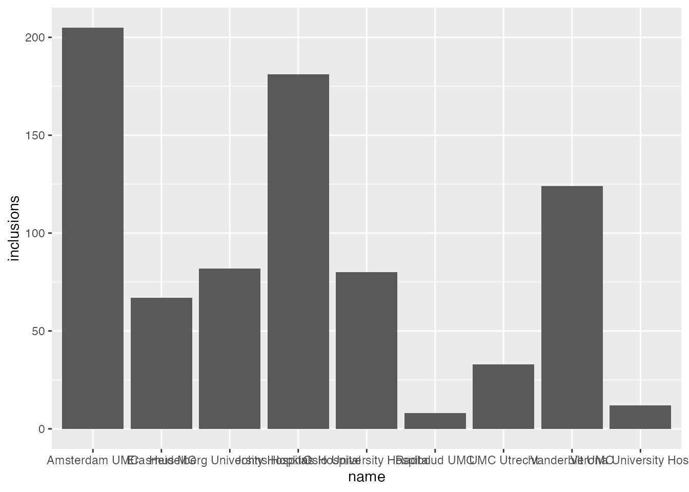
First, we will remove some of the chart junk.
theme_boers <- function(){
theme(text=element_text(family="Corbel", colour="black"),
      #define font
      plot.margin = margin(0.2,1,0,0,"cm"),
      #prevent x axis labels from being cut off
      plot.title = element_text(size=20),
      #text size of the title
      panel.grid.major = element_blank(),
      panel.grid.minor = element_blank(),
      #we do not want automatic grid lines in the background
      axis.text.x=element_text(size=20, colour="black"),
      axis.text.y=element_text(size=20, colour="black"),
      axis.title.x = element_text(size=20),
      axis.title.y = element_text(size=20),
      #define the size of the tick labels and axis titles
      axis.line = element_line(colour = 'black', linewidth = 0.25),
      axis.ticks = element_line(colour = "black", linewidth = 0.25),
      #specify thin axes
      axis.ticks.length = unit(4, "pt"),
      axis.minor.ticks.length = unit(2, "pt"))
  #minor ticks should be shorter than major ticks
}ggplot(data=inclusion_data, aes(name, inclusions)) +
theme_minimal() + theme_boers() +
geom_col()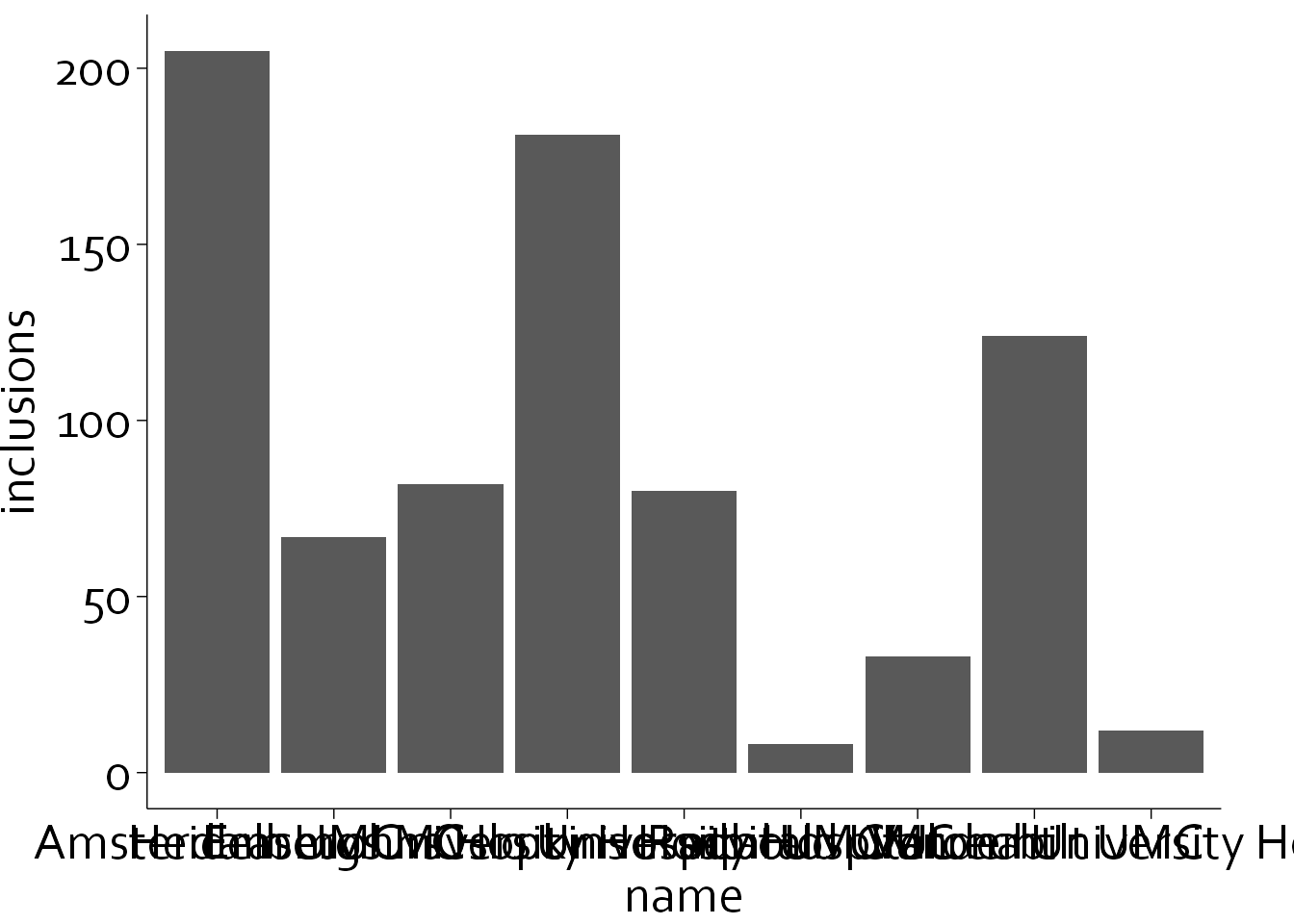
To make the names, more legible, we will flip the axes:
ggplot(data=inclusion_data, aes(name, inclusions)) +
  theme_minimal() + theme_boers() +
geom_col() + coord_flip()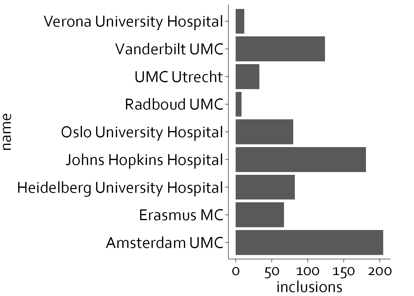
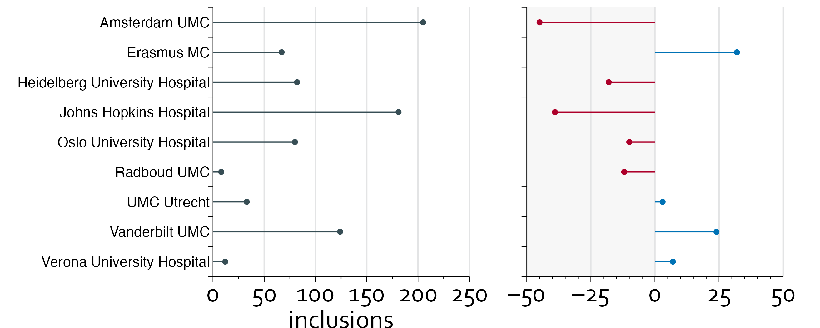
This is better, but there is still a lot of unnecessary non-data ink, i.e., the bar itself. We will replace the bar chart with a so-called lollipop plot, and we will place the centers in alphabetical order.
inclusion_data <- inclusion_data[order(inclusion_data$name),]
inclusion_data$row <- nrow(inclusion_data):1

ggplot(data=inclusion_data, aes(x=inclusions, y=row)) +
  theme_minimal() + theme_boers() +
  geom_point() + geom_segment(aes(x=0, xend=inclusions, y=row, yend=row))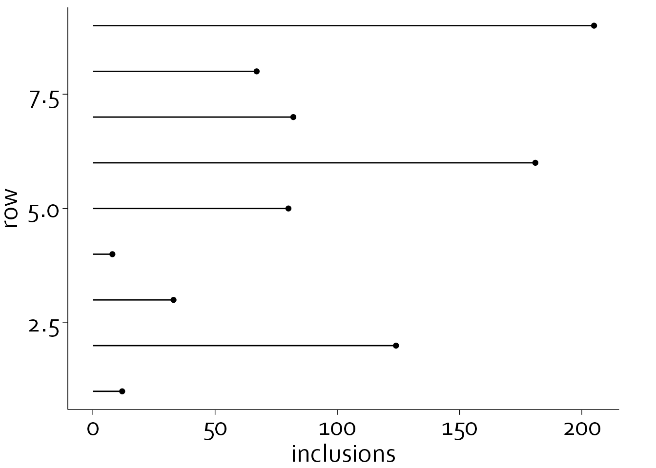
gg1 <- ggplot(data=inclusion_data, aes(x=inclusions, y=row-0.5)) +
   annotate(geom="segment", x=seq(50,250,by=50), xend=seq(50,250,by=50),
            y=0, yend=nrow(inclusion_data), col="#E3E4E5") +
  theme_minimal() + theme_boers() +
  theme(plot.margin = margin(0.2,1,0,5,"cm")) +
  geom_point(colour="#374e55") + geom_segment(aes(x=0, xend=inclusions,
                                  y=row-0.5, yend=row-0.5), colour="#374e55") +
  coord_cartesian(xlim=c(0,250), ylim=c(0,nrow(inclusion_data)), clip = "off") +
  scale_x_continuous(breaks=seq(0,250,by=50),
                       labels=seq(0,250,by=50),
                     minor_breaks = seq(0,250,by=25),
                       expand = c(0,0)) +
  scale_y_continuous(breaks=seq(0,nrow(inclusion_data),by=1),
                     labels=rep("",10),
                     expand=c(0,0)) +
  annotate("text", x=-3, y=inclusion_data$row-0.5, label=inclusion_data$name,
           hjust=1) + ylab("") +
    guides(x = guide_axis(minor.ticks = TRUE))

gg1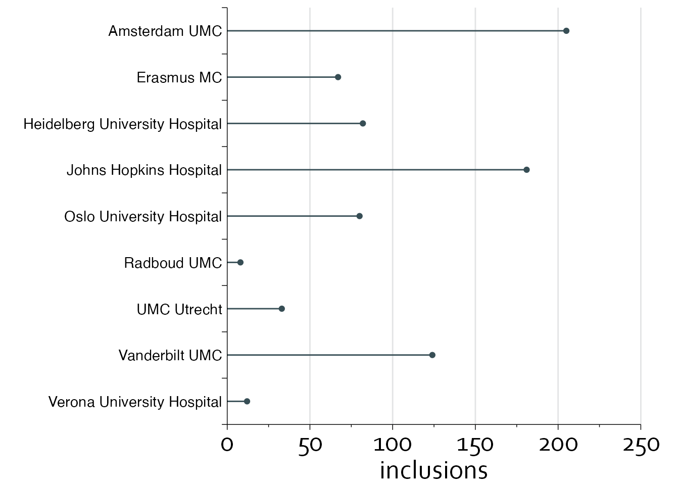
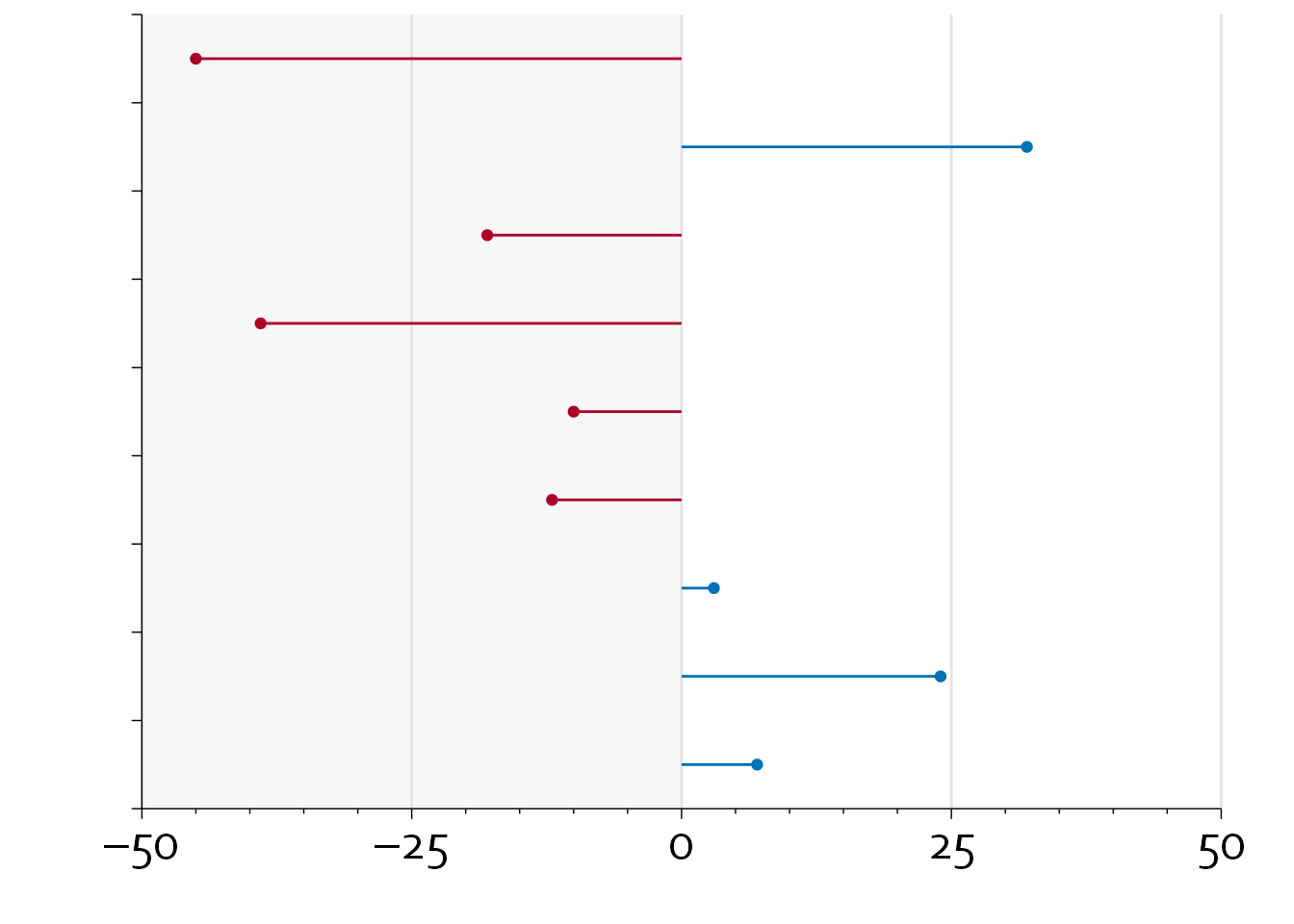
inclusion_data$diff_col <- with(inclusion_data, ifelse(diff<0, "#ad002a", "#0072b5"))
gg2 <- ggplot(data=inclusion_data, aes(x=diff, y=row-0.5)) +
  annotate(geom="rect", xmin=-50, xmax=0, ymin=0, ymax=nrow(inclusion_data),
           fill="#E3E4E5", alpha=0.3) +
   annotate(geom="segment", x=seq(-50,50,by=25), xend=seq(-50,50,by=25),
            y=0, yend=nrow(inclusion_data), colour="#E3E4E5") +
  theme_minimal() + theme_boers() +
  theme(plot.margin = margin(0.2,1,0,1,"cm")) +
  geom_point(colour=inclusion_data$diff_col) +
  geom_segment(aes(x=0, xend=diff, y=row-0.5, yend=row-0.5),
               colour=inclusion_data$diff_col) +
  coord_cartesian(xlim=c(-50,50), ylim=c(0,nrow(inclusion_data)),
                  clip = "off") +
  scale_x_continuous(breaks=seq(-50,50,by=25),
                       labels=c("–50", "–25", "0", "25", "50"),
                     minor_breaks = seq(-50, 50, by=5),
                       expand = c(0,0)) +
  scale_y_continuous(breaks=seq(0,nrow(inclusion_data),by=1),
                     labels=rep("",10),
                     expand=c(0,0)) +
  ylab("") + xlab("") + scale_color_manual() +
  guides(x = guide_axis(minor.ticks = TRUE))

gg2