(Adjusted) survival curves
Randomized trials and observational studies frequently present survival curves to show time-to-event outcomes, and allow comparisons between two or more groups.
In this chapter, you will learn how to:
- Plot Kaplan-Meier curves
- Plot adjusted (‘confounding-corrected’) survival curves, and the difference between two survival curves over time, using flexible parametric survival models
- Plot time-varying hazard ratios, which can be useful when the proportional hazards is violated
- Censoring
- Competing risks
- Immortal time bias
- Clustering
In this chapter, we’ll use data from 2982 patients with primary breast cancer who were included in the Rotterdam tumor bank. Our primary comparison is between patients who did and did not receive hormonal treatment
── Attaching core tidyverse packages ──────────────────────── tidyverse 2.0.0 ──
✔ dplyr     1.1.4     ✔ readr     2.1.5
✔ forcats   1.0.0     ✔ stringr   1.5.1
✔ ggplot2   3.5.1     ✔ tibble    3.2.1
✔ lubridate 1.9.4     ✔ tidyr     1.3.1
✔ purrr     1.0.2
── Conflicts ────────────────────────────────────────── tidyverse_conflicts() ──
✖ dplyr::filter() masks stats::filter()
✖ dplyr::lag()    masks stats::lag()
ℹ Use the conflicted package (<http://conflicted.r-lib.org/>) to force all conflicts to become errorsLoading required package: Hmisc
Attaching package: 'Hmisc'
The following objects are masked from 'package:dplyr':
src, summarize
The following objects are masked from 'package:base':
format.pval, unitsLoading required package: ggpubr
Attaching package: 'survminer'
The following object is masked from 'package:survival':
myeloma| pid | year | age | meno | size | grade | nodes | pgr | er | hormon | chemo | rtime | recur | dtime | death | |
|---|---|---|---|---|---|---|---|---|---|---|---|---|---|---|---|
| 1393 | 1 | 1992 | 74 | 1 | <=20 | 3 | 0 | 35 | 291 | 0 | 0 | 1799 | 0 | 1799 | 0 |
| 1416 | 2 | 1984 | 79 | 1 | 20-50 | 3 | 0 | 36 | 611 | 0 | 0 | 2828 | 0 | 2828 | 0 |
| 2962 | 3 | 1983 | 44 | 0 | <=20 | 2 | 0 | 138 | 0 | 0 | 0 | 6012 | 0 | 6012 | 0 |
| 1455 | 4 | 1985 | 70 | 1 | 20-50 | 3 | 0 | 0 | 12 | 0 | 0 | 2624 | 0 | 2624 | 0 |
| 977 | 5 | 1983 | 75 | 1 | <=20 | 3 | 0 | 260 | 409 | 0 | 0 | 4915 | 0 | 4915 | 0 |
| 617 | 6 | 1983 | 52 | 0 | <=20 | 3 | 0 | 139 | 303 | 0 | 0 | 5888 | 0 | 5888 | 0 |
First, we’ll plot Kaplan-Meier curve to show the unadjusted association between hormonal therapy and overall survival.
theme_boers <- function(){
theme(text=element_text(family="Corbel", colour="black"),
      plot.margin = margin(0.2,1,0,0,"cm"), #prevent x axis labels from being cut off
      plot.title = element_text(size=20),
      panel.grid.major = element_blank(),
      panel.grid.minor = element_blank(),
      axis.text.x=element_text(size=20, colour="black"),
      axis.text.y=element_text(size=20, colour="black"),
      axis.title.x = element_text(size=20),
      axis.title.y = element_text(size=20),
      axis.line = element_line(colour = 'black', linewidth = 0.25),
      axis.ticks = element_line(colour = "black", linewidth = 0.25),
      axis.ticks.length = unit(4, "pt"),
      axis.minor.ticks.length = unit(2, "pt"))
}

os_summary <- surv_summary(survfit(Surv(dtime, death)~hormon,
                                   data=os_dat), data=os_dat)
os_summary <- as.data.frame(os_summary)

os_temp <- os_summary[1,]
os_temp[2,] <- os_temp[1,]

os_temp$time <- 0
os_temp$n.risk <- c(2643, 339)
os_temp$strata <- c("hormon=0", "hormon=1")
os_temp$hormon <- c(0,1)

os_summary <- rbind(os_temp, os_summary)

os_summary$time <- os_summary$time/365.24

os_summary_0 <- subset(os_summary, hormon==0 & time<=10)
os_summary_1 <- subset(os_summary, hormon==1 & time<=10)
bg_line_dat <- data.frame("x"=rep(0,6), "xend"=rep(10.5,6),
"y"=seq(0,1,by=0.2), "yend"=seq(0,1,by=0.2))
gg <- ggplot(data=os_summary_0, aes(time,surv)) +
theme_minimal() + theme_boers() +
geom_segment(data=bg_line_dat, aes(x=x, xend=xend,
y=y, yend=yend),
col="#e3e4e5") +
geom_step(colour="#374e55",
linewidth=1) +
geom_ribbon(aes(ymin=lower, ymax=upper), fill="#374e5530") +
geom_step(data=os_summary_1, aes(time,surv),
colour="#df8f44", linewidth=1) +
geom_ribbon(data=os_summary_1,
aes(ymin=lower, ymax=upper), fill="#df8f4430") +
#geom_smooth(method="gam", formula = y ~ s(x, bs = "cs")) +
annotate("text", x=6, y=0.815, label="No hormonal therapy",
fontface=2, colour="#374e55") +
annotate("text", x=3, y=0.615, label="Hormonal therapy",
fontface=2, colour="#df8f44") +
scale_x_continuous(breaks=seq(0,10,by=1),
labels=seq(0,10,by=1),
minor_breaks = seq(0,10,by=0.5),
expand = c(0,0)) +
scale_y_continuous(breaks=seq(0,1,by=0.2),
labels=c(0,0.2,0.4,0.6,0.8,"1.0"),
minor_breaks = seq(0,1,by=0.1),
expand = c(0,0)) +
guides(x = guide_axis(minor.ticks = TRUE),
y = guide_axis(minor.ticks = TRUE)) +
coord_cartesian(xlim=c(0,10.5), ylim=c(0,1), clip = "off") +
xlab("Time after diagnosis (years)") + ylab("Survival probability")
gg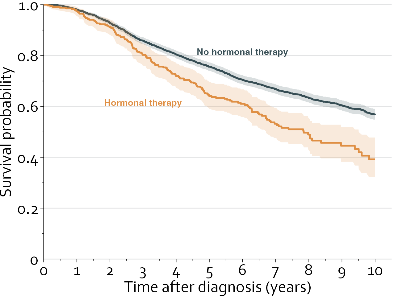
We’ll use Cox regression to estimate the unadjusted hazard ratio:
Cox Proportional Hazards Model

cph(formula = Surv(dtime, death) ~ hormon, data = os_dat)

                       Model Tests     Discrimination
                                              Indexes
Obs      2982    LR chi2     21.12     R2       0.007
Events   1272    d.f.            1    R2(1,2982)0.007
Center 0.0471    Pr(> chi2) 0.0000    R2(1,1272)0.016
                 Score chi2  23.69     Dxy      0.042
                 Pr(> chi2) 0.0000

       Coef   S.E.   Wald Z Pr(>|Z|)
hormon 0.4144 0.0853 4.86 <0.0001 [1] 1.280451 1.513462 1.788877The unadjusted (‘crude’) hazard ratio is 1.51 (95% confidence interval, 1.28 to 1.79; P<0.0001), indicating that hormonal therapy is associated with shorter overall survival. We’ll now adjust for several potential confounders, including age, menopausal state, and tumor size:
cph_os <- cph(Surv(dtime, death) ~ hormon + rcs(age, 4) + meno +
                 size + grade + rcs(log(nodes+1),4) +
                 rcs(log(pgr+1),4) + rcs(log(er+1), 4),
               data=os_dat)

dd <- datadist(os_dat)
options(datadist = "dd")

summary(cph_os)
Effects Response : Surv(dtime, death)
Factor Low High Diff. Effect S.E. Lower 0.95 Upper 0.95
hormon 0 1.00 1.00 -0.269790 0.090741 -0.44764 -0.09194
Hazard Ratio 0 1.00 1.00 0.763540 NA 0.63914 0.91216
age 45 65.00 20.00 -0.145610 0.142480 -0.42487 0.13364
Hazard Ratio 45 65.00 20.00 0.864490 NA 0.65386 1.14300
meno 0 1.00 1.00 0.372610 0.127110 0.12347 0.62175
Hazard Ratio 0 1.00 1.00 1.451500 NA 1.13140 1.86220
grade 2 3.00 1.00 0.276760 0.071245 0.13713 0.41640
Hazard Ratio 2 3.00 1.00 1.318900 NA 1.14700 1.51650
nodes 0 4.00 4.00 0.973510 0.074782 0.82694 1.12010
Hazard Ratio 0 4.00 4.00 2.647200 NA 2.28630 3.06510
pgr 4 198.00 194.00 -0.376860 0.099832 -0.57252 -0.18119
Hazard Ratio 4 198.00 194.00 0.686020 NA 0.56410 0.83428
er 11 202.75 191.75 0.010873 0.091326 -0.16812 0.18987
Hazard Ratio 11 202.75 191.75 1.010900 NA 0.84525 1.20910
size - 20-50:<=20 1 2.00 NA 0.296260 0.066396 0.16613 0.42639
Hazard Ratio 1 2.00 NA 1.344800 NA 1.18070 1.53170
size - >50:<=20 1 3.00 NA 0.531100 0.093384 0.34807 0.71413
Hazard Ratio 1 3.00 NA 1.700800 NA 1.41630 2.04240 The adjusted hazard ratio for hormonal therapy is 0.76 (95% CI, 0.64 to 0.91), indicating that hormonal therapy is associated with longer overall survival.